Computational Grid¶

Coordinate Systems¶

ChiDG supports two coordinate systems: Cartesian and Cylindrical. In the code, many things are referred to only by coordinate index. The convention for these indices is defined here as:

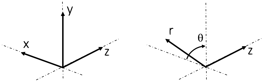
\[ \begin{align}\begin{aligned}(x,y,z) \rightarrow (1,2,3)\\(r, \theta, z) \rightarrow (1,2,3)\end{aligned}\end{align} \]

Additionally, effort has been put forth to represent data in a manner consistent with vector-calculus. For example, test function gradient components are computed as:

\[ \begin{align}\begin{aligned}\nabla \psi = \frac{\partial \psi}{\partial x}\hat{x} + \frac{\partial \psi}{\partial y} \hat{y} + \frac{\partial \psi}{\partial z} \hat{z}\\\nabla \psi = \frac{\partial \psi}{\partial r}\hat{r} + \frac{1}{r}\frac{\partial \psi}{\partial \theta} \hat{\theta} + \frac{\partial \psi}{\partial z} \hat{z}\end{aligned}\end{align} \]

The transformation between Cartesian and Cylindrical coordinates is given by

\[\begin{split}x &= r cos(\theta) \quad\quad\quad r &= \sqrt{x^2 + y^2} \\ y &= r sin(\theta) \quad\quad\quad \theta &= \text{atan2}(y,x) \\ z &= z \quad\quad\quad\quad\quad \: \: z &= z\end{split}\]

Mesh¶

A mesh_t instance contains the entire description of the computational grid for the local processor. A mesh_t conatains an array of domain_t objects, one for each block. A mesh_t object also contains boundary condition geometry, located in the bc_patch_group component. The bc_patch_group objects are independent of the domains. A given bc_patch_group could potentially include references to faces on multiple domain objects.

type :: mesh_t

    type(domain_t),         allocatable :: domain(:)
    type(bc_patch_group_t), allocatable :: bc_patch_group(:)

contains

end type mesh_t

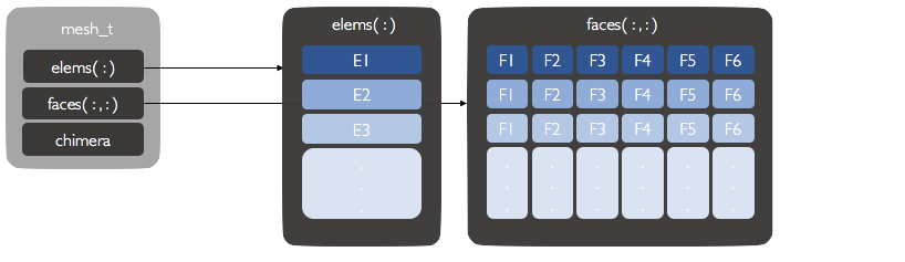
Domain¶

The domain_t data structure contains an entire geometry description for a single domain. This exists as an array of element_t types, and array of face_t types, and a chimera_t instance. An element_t exists for every element in the domain_t domain. For a given element_t, a face_t instance exists for each face.

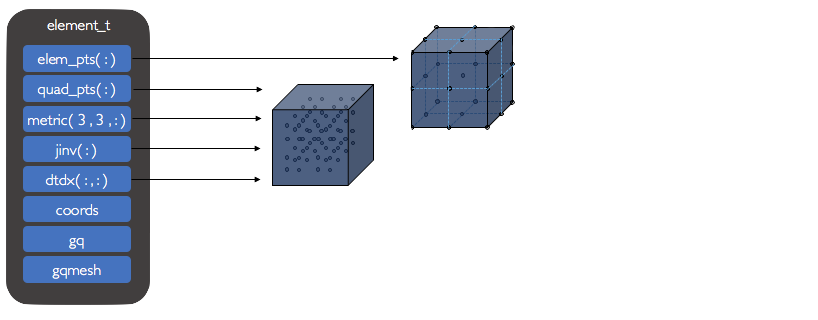
Element¶

An element_t instance contains information needed by the framework and also general information that could be useful to users. This includes:

node_coords(:,:)      An array of points defining the undeformed element in real space(cartesian, cylindrical, etc.). [nnodes, ncoords]
node_coords_def(:,:)  An array of points defining the deformed element in real space(cartesian, cylindrical, etc.). [nnodes, ncoords]
node_coords_vel(:,:)  An array of points defining the element in real space(cartesian, cylindrical, etc.). [nnodes, ncoords]
interp_coords(:)      An array of points defining the undeformed coordinates of each volume interpolation node in real space.
interp_coords_def(:)  An array of points defining the deformed coordinates of each volume interpolation node in real space.
interp_coords_vel(:)  An array of points defining the coordinate velocities of each volume interpolation node in real space.
metric(3,3,:)         An array, defining for each interpolation node, a matrix of element metric values.
jinv(:)               An array of inverse element jacobian values at each volume interpolation node.
jinv_def(:)           An array of inverse element jacobian values at each volume quadrature node.
grad1(:,:)            An array of gradients of the basis functions with respect to physical coordinates at volume quadrature nodes.

Metric terms¶

The transformation of a differential volume in physical space(\([x,y,z]\) or \([r,\theta,z]\)) to reference space(\([\xi,\eta,\zeta] = [-1,1]\) is computed as

\[\begin{split}\begin{pmatrix} dx \\ dy \\ dz \end{pmatrix} = \begin{pmatrix} x_\xi \quad x_\eta \quad x_\zeta \\ y_\xi \quad y_\eta \quad y_\zeta \\ z_\xi \quad z_\eta \quad z_\zeta \end{pmatrix} \begin{pmatrix} d\xi \\ d\eta \\ d\zeta \end{pmatrix} \quad \quad \quad \begin{pmatrix} dr \\ rd\theta \\ dz \end{pmatrix} = \begin{pmatrix} r_\xi \quad r_\eta \quad r_\zeta \\ r\theta_\xi \quad r\theta_\eta \quad r\theta_\zeta \\ z_\xi \quad z_\eta \quad z_\zeta \end{pmatrix} \begin{pmatrix} d\xi \\ d\eta \\ d\zeta \end{pmatrix}\end{split}\]

The terms \(\partial \vec{x}/\partial \vec{\xi}\) are computed from the polynomial expansion representing the element coordinates as

\[x = \sum \psi \hat{x} \quad\rightarrow\quad \frac{\partial x}{\partial \xi} = \sum \frac{\partial \psi}{\partial \xi} \hat{x}\]

The element metric terms are obtained by inverting the matrices \(\partial \vec{x}/\partial \vec{\xi}\) to give

\[\begin{split}\mathcal{T} = \begin{pmatrix} \xi_x \quad \xi_y \quad \xi_z \\ \eta_x \quad \eta_y \quad \eta_z \\ \zeta_x \quad \zeta_y \quad \zeta_z \end{pmatrix} \quad \quad \quad \mathcal{T} = \begin{pmatrix} \xi_r \quad \xi_\theta \quad \xi_z \\ \eta_r \quad \eta_\theta \quad \eta_z \\ \zeta_r \quad \zeta_\theta \quad \zeta_z \end{pmatrix}\end{split}\]

Note, that the cylindrical element transformation matrix has \(r\)-scaling included implicitly since it was computed by inverting the mapping constructed previously. The metric terms are defined at each quadrature point in the metric(:,:,:) component of a given element_t. To access the matrix of metric components for a given quadrature node igq, the component can be used as

metric(:,:,igq)

This returns the metric components(Cartesian or Cylindrical) at the quadrature node in a 3x3 matrix as

\[\begin{split}\begin{pmatrix} \xi_x \quad \xi_y \quad \xi_z \\ \eta_x \quad \eta_y \quad \eta_z \\ \zeta_x \quad \zeta_y \quad \zeta_z \end{pmatrix} \quad \quad \quad \begin{pmatrix} \xi_r \quad \xi_\theta \quad \xi_z \\ \eta_r \quad \eta_\theta \quad \eta_z \\ \zeta_r \quad \zeta_\theta \quad \zeta_z \end{pmatrix}\end{split}\]

Alternatively, a given metric term can be accessed for the set of quadrature nodes as

metric(1,1,:)

which would return a 1D array of values for (\(\xi_x\) or \(\xi_r\)) corresponding to each quadrature node in the set.

The inverse element jacobian terms(Cartesian or Cylindrical) jinv(:) are defined at each quadrature node as

\[ \begin{align}\begin{aligned}J^{-1} = ( x_\xi y_\eta z_\zeta - x_\eta y_\xi z_\zeta - x_\xi y_\zeta z_\eta + x_\zeta y_\xi z_\eta + x_\eta y_\zeta z_\xi - x_\zeta y_\eta z_\xi )\\J^{-1} = r ( r_\xi \theta_\eta z_\zeta - r_\eta \theta_\xi z_\zeta - r_\xi \theta_\zeta z_\eta + r_\zeta \theta_\xi z_\eta + r_\eta \theta_\zeta z_\xi - r_\zeta \theta_\eta z_\xi )\end{aligned}\end{align} \]

Gradients¶

Gradients of basis functions with respect to the reference coordinates are not dependent on the physical coordinate system. So, any calculations of the terms \(\partial \psi/\partial \vec{\xi}\) do not need to be modified with a change from one physical coordinate system to another. These gradients are defined on a defined in a quadrature instance associated with an element in the component element%gq%vol. For example, the component element%gq%vol%ddxi gives:

\[\begin{split}\frac{\partial \psi_{igq, imode}}{\partial \xi} = \begin{pmatrix} \frac{\partial \psi_{1,1}}{\partial \xi} & \frac{\partial \psi_{1,2}}{\partial \xi} & \cdots & \frac{\partial \psi_{1,N}}{\partial \xi} \\ \frac{\partial \psi_{2,1}}{\partial \xi} & \frac{\partial \psi_{2,2}}{\partial \xi} & \cdots & \frac{\partial \psi_{2,N}}{\partial \xi} \\ \vdots & \vdots & \vdots & \vdots \\ \frac{\partial \psi_{{ngq},1}}{\partial \xi} & \frac{\partial \psi_{{ngq},2}}{\partial \xi} & \cdots & \frac{\partial \psi_{{ngq},N}}{\partial \xi} \\ \end{pmatrix}\end{split}\]

Gradients with respect to the physical coordinate system do change depending on the coordinate system being used. The gradient for Cartesian and Cylindrical coordinates is

\[\begin{split}\nabla f &= \frac{\partial f}{\partial x}\hat{x} + \frac{\partial f}{\partial y}\hat{y} + \frac{\partial f}{\partial z}\hat{z} \\ \nabla f &= \frac{\partial f}{\partial r}\hat{r} + \frac{1}{r}\frac{\partial f}{\partial \theta}\hat{\theta} + \frac{\partial f}{\partial z}\hat{z}\end{split}\]

The coordinate transformation for the gradient from reference space to physical space is computed using the transpose of the element metric matrix as

\[\nabla_x \psi = \mathcal{T}^T \nabla_\xi \psi\]

For the Cartesian and Cylindrical coordinate systems, these are expanded as

\[\begin{split}\nabla_{\vec{x}} \psi = \begin{bmatrix} \xi_x & \eta_x & \zeta_x \\ \xi_y & \eta_y & \zeta_y \\ \xi_z & \eta_z & \zeta_z \\ \end{bmatrix} \begin{bmatrix} \psi_\xi \\ \psi_\eta \\ \psi_\zeta \end{bmatrix} \\ \nabla_{\vec{r}} \psi = \begin{bmatrix} \xi_r & \eta_r & \zeta_r \\ \xi_\theta & \eta_\theta & \zeta_\theta \\ \xi_z & \eta_z & \zeta_z \\ \end{bmatrix} \begin{bmatrix} \psi_\xi \\ \psi_\eta \\ \psi_\zeta \end{bmatrix}\end{split}\]

Note that the terms \(\nabla_{\vec{x}} \psi\) and \(\nabla_{\vec{r}} \psi\) are the gradient vectors and not the directional derivatives. For the Cartesian coordinate system, these things are identical. For the cylindrical coordinate system, they are not.

Gradients of basis functions with respect to the pysical coordinate system in an element_t can be accessed in the grad1(:,:), grad2(:,:), and grad3(:,:) components. For example, the element%grad1 component contains the gradient along the 1st physical coordinate for all basis functions at all quadrature nodes as:

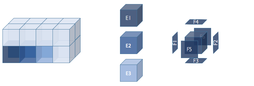
\[\begin{split}\nabla_1 \psi_{ngq, nmode} = \begin{pmatrix} \nabla_1 \psi_{1,1} & \nabla_1 \psi_{1,2} & \cdots & \nabla_1 \psi_{1,N} \\ \nabla_1 \psi_{2,1} & \nabla_1 \psi_{2,2} & \cdots & \nabla_1 \psi_{2,N} \\ \vdots & \vdots & \vdots & \vdots \\ \nabla_1 \psi_{{ngq},1} & \nabla_1 \psi_{{ngq},2} & \cdots & \nabla_1 \psi_{{ngq},N} \\ \end{pmatrix}\end{split}\]

Face¶

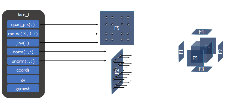
Face metrics¶

Metric terms for the face_t data structure are defined exactly the same as for the element_t data structure. The difference is that the metric and jinv components of face_t return values for boundary quadrature nodes. This contrasts the element_t structure, which returns values for volume quadrature nodes.

Face normals¶

\[\vec{x} = [x, y, z] \quad \vec{\xi} = [\xi, \eta, \zeta]\]

Face normal vectors are stored for each face quadrature node. The component norm is the face normal vector with respect to computational coordinates on a reference element (\(\xi\), \(\eta\), \(\zeta\)) as

\[\vec{n}_{\xi_k} = \frac{\partial \vec{x}}{\partial \xi_i} \times \frac{\partial \vec{x}}{\partial \xi_j}\]

where \(\xi_i\) and \(\xi_j\) are the in-place coordinates of face \(\xi_k\). In this was, the normal vectors for \(\xi\), \(\eta\), and \(\zeta\) faces are defined respectively as

\[ \begin{align}\begin{aligned}\vec{n}_\xi = \frac{\partial \vec{x}}{\partial \eta} \times \frac{\partial \vec{x}}{\partial \zeta} = [ y_\eta z_\zeta - y_\zeta z_\eta, \quad x_\zeta z_\eta - x_\eta z_\zeta, \quad x_\eta y_\zeta - x_\zeta y_\eta] = [ \xi_x, \quad \xi_y, \quad \xi_z ]\\\vec{n}_\eta = \frac{\partial \vec{x}}{\partial \zeta} \times \frac{\partial \vec{x}}{\partial \xi} = [ y_\zeta z_\xi - y_\xi z_\zeta, \quad x_\xi z_\zeta - x_\zeta z_\xi, \quad x_\zeta y_\xi - x_\xi y_\zeta ] = [ \eta_x, \quad \eta_y, \quad \eta_z ]\\\vec{n}_\zeta = \frac{\partial \vec{x}}{\partial \xi} \times \frac{\partial \vec{x}}{\partial \eta} = [ y_\xi z_\eta - y_\eta z_\xi, \quad x_\eta z_\xi - x_\xi z_\eta, \quad x_\xi y_\eta - x_\eta y_\xi] = [ \zeta_x, \quad \zeta_y, \quad \zeta_z ]\end{aligned}\end{align} \]

Applying the above formula to element faces produces normal vectors that are inward facing for \(\xi = -1\) faces and outward facing for \(\xi = 1\) faces. Inward facing vectors are negated so that all resultant normal vectors in the norm component are outward facing. This applied to \(\eta\) and \(\zeta\) faces as well.

Unit normal vectors can be accessed in the unorm component and are computed as

\[\hat{n}_{\xi_i} = \frac{\vec{n}_{\xi_i}}{||\vec{n}_{\xi_i}||_2}\]

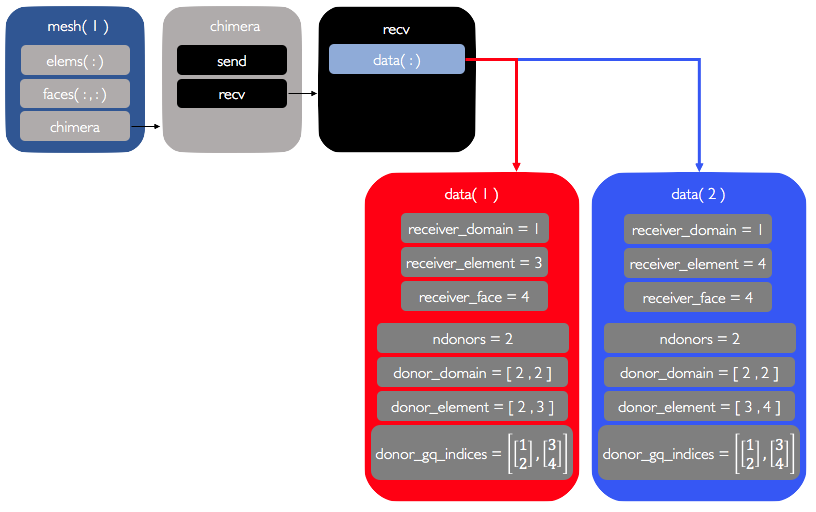
Chimera Interfaces¶

Each domain_t instance contains a domain%chimera component that holds all information regarding chimera communication for that particular mesh block. This takes the form of chimera_receiver and chimera_donor components. Currently, only the chimera_receiver is utilized. chimera_donor will be used to facilitate communication between processors for parallel code execution.

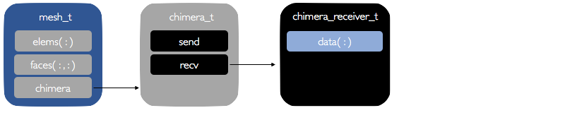
In a given domain_t, every face that gets information from a separate block is designated as a CHIMERA face, it is assigned an integer ID face%ChiID, and it gets an entry in the domain%chimera%recv%data components. It can be accessed as

domain%chimera%recv%data(ChiID)

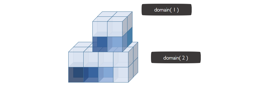
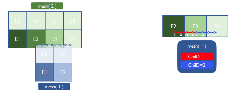
Example¶

Consider an example with two domains, as shown below. domain(1) contains four elements. domain(2) contains eight elements. domain(1) overlaps with domain(2). In particular, the top faces of elements E3 and E4 lie inside domain(2). These faces are designated as CHIMERA faces and are given a mesh-global chimera ID. The top face of E3 is given the ID ChiID=1 and the top face of E4 is given the ID ChiID=2.

Each CHIMERA face has its own set of chimera information, which can be accessed via domain%chimera%recv%data(ChiID). This is shown below for the two faces in this example.